A Mini Tour of Open-source tools for Transportation Planning & Engineering
ITE UWindsor Chapter
November 30th, 2023
Photo by Norali Nayla on Unsplash and snowflakes by Emil Hvitfeldt
About me
- Data Scientist at Presage Group
- Formerly:
- Postdoctoral Fellow at University of Windsor
- Data Analytics Instructor at St. Clair College
Routing, Accessibility, and Transit
stplanr: Sustainable Transport Planning
Tools for transport planning with an emphasis on spatial transport data and non-motorized modes
Origin-desination data
Flows
Origin-desination data
Spatial geometry
Network
Plot the network
Routing
Routing output
r5r: Rapid Realistic Routing with R5 in R
Setup
Location
Calculate accessibility
departure_datetime <- as.POSIXct("29-11-2023 14:00:00",
format = "%d-%m-%Y %H:%M:%S")
# calculate accessibility
access <- accessibility(r5r_core = r5r_core,
origins = points,
destinations = points,
opportunities_colnames = c("schools", "healthcare"),
mode = c("WALK", "TRANSIT"),
max_walk_time = 30,
departure_datetime = departure_datetime,
decay_function = "step",
cutoffs = 20
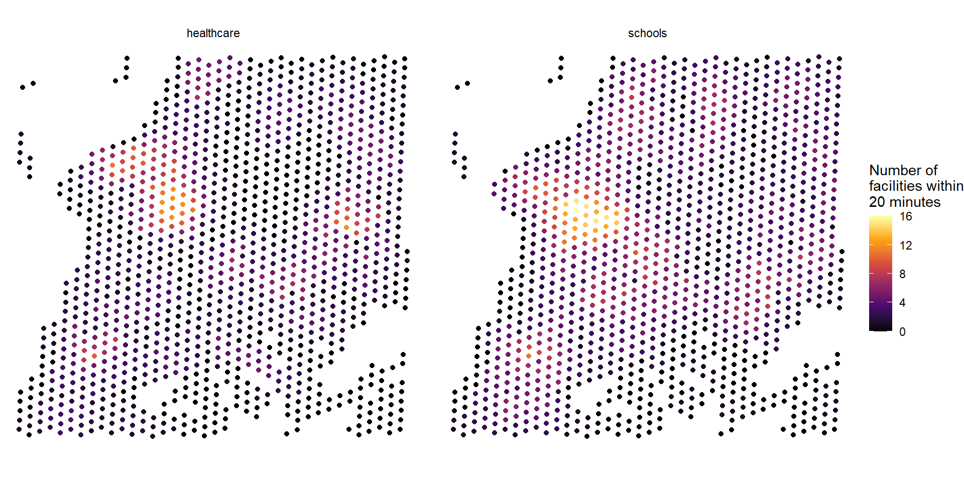
)Plot accessibility: static plot
Plot accessibility: static plot

Plot accessibility: interactive plot
access_sf_schools <- access_sf |>
dplyr::filter(opportunity == "schools")
pal <- colorNumeric(
palette = "magma",
domain = access_sf_schools$accessibility)
access_sf_schools |>
leaflet() |>
addTiles() |>
addCircles(color = ~pal(accessibility), group = "Points") |>
addLegend("bottomright", pal = pal, values = ~accessibility,
title = "Access within 20 min.",
opacity = 1
) |>
addLayersControl(overlayGroups = c("Points"),
options = layersControlOptions(collapsed = FALSE))Plot accessibility: interactive plot
Statistics Canada has estimated accessibility for all of Canada
Tidytransit: Transit Windsor
# Install with: install.packages("tidytransit")
library(tidytransit)
library(sf)
gtfs <- read_gtfs("https://opendata.citywindsor.ca/Uploads/google_transit.zip")
names(gtfs) [1] "agency" "shapes" "trips" "stops"
[5] "stop_times" "routes" "calendar" "calendar_dates"
[9] "feed_info" "fare_attributes" "fare_rules" "." Code
# get all service_ids for mondays
all_mondays <- gtfs$calendar %>%
filter(monday == 1) %>%
pull(service_id)
# select trips on mondays
selected_trips <- gtfs$routes %>%
left_join(gtfs$trips, by = "route_id") %>%
filter(service_id %in% all_mondays) # only take trips on mondays
# get linestrings for routes
selected_shapes <- gtfs$shapes %>%
filter(shape_id %in% unique(selected_trips$shape_id) )
shapes <- shapes_as_sf(selected_shapes)
# df with linestring, start and end time
windsor_transit <- selected_trips %>%
left_join (gtfs$stop_times, by = "trip_id") %>%
arrange(trip_id, stop_sequence) %>%
select(trip_id, route_id, shape_id, route_short_name, departure_time) %>%
group_by(trip_id, route_id, route_short_name, shape_id) %>%
summarise(starttime = first(departure_time),
endtime = last(departure_time)) %>%
left_join(shapes, by = "shape_id") %>%
st_as_sf() %>%
mutate(start_timestamp = as.numeric(as.POSIXct(starttime, format="%H:%M:%S"))) %>%
mutate(end_timestamp = as.numeric(as.POSIXct(endtime, format="%H:%M:%S"))) %>%
filter(!is.na(start_timestamp)) %>%
filter(!is.na(end_timestamp)) # for simlicity dates greater than 24h are ignored
windsor_transitPlot
Traffic flow and Simulation
Photo by <a https://unsplash.com/@chuttersnap“>CHUTTERSNAP on Unsplash
hereR: Download and plot real-time traffic data
Get Windsor polygons
download.file(url = "https://opendata.citywindsor.ca/Uploads/Municipal%20Ward%20Boundaries_UTM83.zip", destfile = "windsor_boundaries.zip")
unzip("windsor_boundaries.zip")
windsor <- sf::st_read("Municipal Ward Boundaries_UTM83.shp")Reading layer `Municipal Ward Boundaries_UTM83' from data source
`D:\ostForTransport\Municipal Ward Boundaries_UTM83.shp' using driver `ESRI Shapefile'
Simple feature collection with 10 features and 3 fields
Geometry type: POLYGON
Dimension: XY
Bounding box: xmin: 325905 ymin: 4677685 xmax: 344156.6 ymax: 4690549
Projected CRS: NAD83 / UTM zone 17NGet speed and jam factor
jam factor: The number between 0.0 and 10.0 indicating the expected quality of travel.
# Install with: install.packages("hereR")
library(hereR)
flows_windsor <- flow(aoi = windsor)
library(leafpop)
library(leafsync)
m1 <- mapview(flows_windsor,
popup = popupTable(flows_windsor,
zcol = c(
"free_flow",
"speed",
"jam_factor",
"confidence"
)
),
zcol = "speed",
layer.name = "speed"
)
m2 <- mapview(flows_windsor,
popup = popupTable(flows_windsor,
zcol = c(
"free_flow",
"speed",
"jam_factor",
"confidence"
)
),
zcol = "jam_factor",
layer.name = "jam_factor"
)
sync(m1, m2)Get speed and jam factor
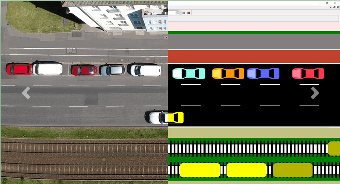
SUMO Simulation of Urban MObility
You may have heard of the popular PTV Vissim microscopic simulation software. SUMO is an open source alternative.

SUMO Features
- Open source - C++
- Automated driving
- Vehicle Communication
- Control the behaviour of simulation objects via Traffic Control Interface (TraCI)
TraCI
Use Python to control simulation

Traffic Simulation with SUMO, NETEDIT, and TraCI
carfollowingmodels: Car Following Models in R
I developed this package for microscopic simulation in R
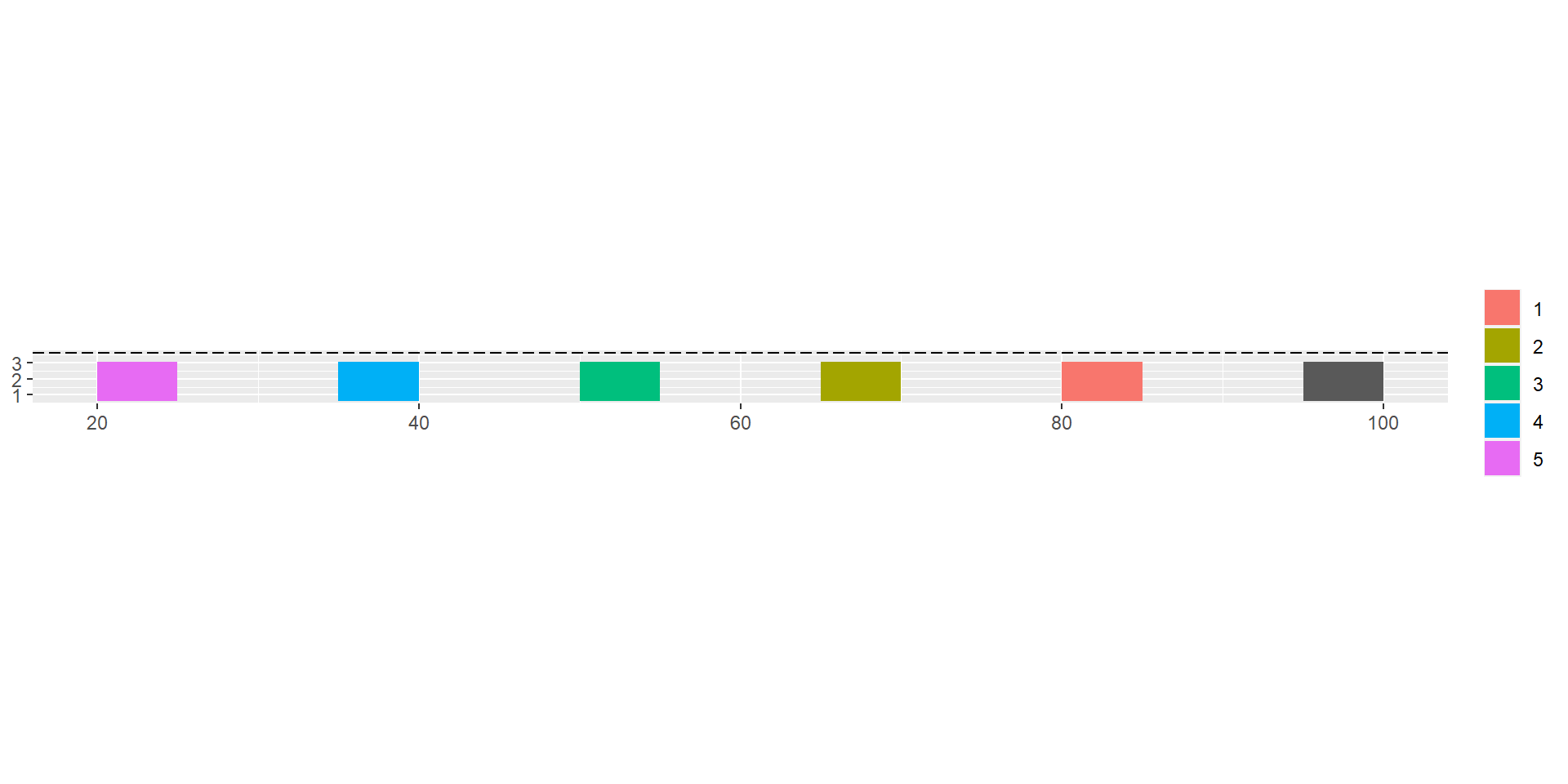
- Example: Five following vehicles:

Example: Provide Wiedemann Model Parameters
# Install with:
# install.packages("devtools")
# devtools::install_github("durraniu/carfollowingmodels")
library(carfollowingmodels)
results_w74d <- simulate_wiedemann74_driver(
resolution=0.1,
N=5,
dfn1=ldf,
xn1="xn1_complete",
vn1="vn1_complete",
bn1="bn1_complete",
xn_first=list(85, 70, 55, 40, 25),
vn_first=list(12, 12, 12, 12, 12),
ln=list(5, 5, 5, 5, 5),
D_MAX=150,
V_MAX=44,
V_DESIRED=14.4,
FAKTORVmult=0.001,
BMAXmult=0.08,
BNULLmult=0.25,
BMIN=-5,
CX=50,
AXadd=2,
BXadd=2,
EXadd=2,
OPDVadd=1.5
)
head(results_w74d)