Predicting Iris Species with ML

Load Packages

We begin by loading all the required packages for ML and visualization.

library(randomForest)
library(caret)
library(ggplot2)
library(dplyr)
library(tidyr)
library(gt)
# NEW
library(quarto)
library(brand.yml)

Code

plot_theme <- theme_brand_ggplot2("_brand.yml")
table_theme <- quarto::theme_brand_gt("_brand.yml")
color_palette <- list(
  discrete1 = c("#6E2DAB", "#49752E", "#FFB300", "#D7263D", "#008B8B"), 
  discrete2 = c("#9B79CD", "#2F4F4F", "#B0C4DE", "#DAA520", "#A52A2A"), 
  sequential1 = c("#EFEFF8", "#C7BDE0", "#9B79CD", "#6E2DAB", "#522180"), 
  sequential2 = c("#EBF5E7", "#B8D3A8", "#82B471", "#49752E", "#30511F"), 
  sequential3 = c("#FFF8E1", "#FFDDA1", "#FFB300", "#CC8C00", "#996600"), 
  diverging1 = c("#A50F15", "#D7263D", "#F49C8F", "#FDF7EC", "#A5D6A7", "#49752E","#284A1A"), 
  diverging2 = c("#522180", "#6E2DAB", "#B6A0D9", "#FDF7EC", "#FFDDA1", "#FFB300","#CC8C00"))
theme_set(plot_theme + theme(
    plot.title = element_text(size = 15),
    axis.text = element_text(size = 12),
    axis.title = element_text(size = 13)
  ))

Load Data

The next step is to load the iris dataset:

data(iris)
iris |> 
    head() |> 
    gt() |> 
    tab_header(title = "Iris Flowers") |> 
    table_theme()

Sepal.Length	Sepal.Width	Petal.Length	Petal.Width	Species
Iris Flowers
5.1	3.5	1.4	0.2	setosa
4.9	3.0	1.4	0.2	setosa
4.7	3.2	1.3	0.2	setosa
4.6	3.1	1.5	0.2	setosa
5.0	3.6	1.4	0.2	setosa
5.4	3.9	1.7	0.4	setosa

Create feature matrix and target vector

X <- iris[, 1:4]
y <- iris$Species

Split the data (70% train, 30% test)

set.seed(42)
train_index <- createDataPartition(y, p = 0.7, list = FALSE)
X_train <- X[train_index, ]
X_test  <- X[-train_index, ]
y_train <- y[train_index]
y_test  <- y[-train_index]

Standardize features

# Calculate mean and sd manually for each column
scaling_params <- data.frame(
  feature = colnames(X_train),
  mean = apply(X_train, 2, mean),
  sd = apply(X_train, 2, sd)
)

# Display scaling parameters
scaling_params |> 
  gt() |> 
  tab_header(title = "Scaling Parameters") |>
  fmt_number(columns = c(mean, sd), decimals = 4) |> 
  table_theme()

feature	mean	sd
Scaling Parameters
Sepal.Length	5.8857	0.8380
Sepal.Width	3.0705	0.4036
Petal.Length	3.8133	1.7924
Petal.Width	1.2162	0.7796

# Apply scaling
X_train_scaled <- scale(X_train, center = scaling_params$mean, scale = scaling_params$sd)
X_test_scaled <- scale(X_test, center = scaling_params$mean, scale = scaling_params$sd)

Train a Random Forest classifier

set.seed(42)
model <- randomForest(x = X_train_scaled, 
                     y = y_train, 
                     ntree = 100, 
                     importance = TRUE)

Make predictions

y_pred <- predict(model, X_test_scaled)

Evaluate the model

accuracy <- sum(y_pred == y_test) / length(y_test)
cat("Model Accuracy:", sprintf("%.2f%%", accuracy * 100), "\n")

Model Accuracy: 93.33%

Classification Report

cat("Classification Report:\n")

Classification Report:

conf_matrix <- confusionMatrix(y_pred, y_test)
conf_matrix

Confusion Matrix and Statistics

            Reference
Prediction   setosa versicolor virginica
  setosa         15          0         0
  versicolor      0         14         2
  virginica       0          1        13

Overall Statistics
                                         
               Accuracy : 0.9333         
                 95% CI : (0.8173, 0.986)
    No Information Rate : 0.3333         
    P-Value [Acc > NIR] : < 2.2e-16      
                                         
                  Kappa : 0.9            
                                         
 Mcnemar's Test P-Value : NA             

Statistics by Class:

                     Class: setosa Class: versicolor Class: virginica
Sensitivity                 1.0000            0.9333           0.8667
Specificity                 1.0000            0.9333           0.9667
Pos Pred Value              1.0000            0.8750           0.9286
Neg Pred Value              1.0000            0.9655           0.9355
Prevalence                  0.3333            0.3333           0.3333
Detection Rate              0.3333            0.3111           0.2889
Detection Prevalence        0.3333            0.3556           0.3111
Balanced Accuracy           1.0000            0.9333           0.9167

Confusion Matrix for Plotting

cm <- table(Actual = y_test, Predicted = y_pred)
cm_df <- as.data.frame(cm)

Plot 1: Confusion Matrix

confusion_plot <- ggplot(cm_df, aes(x = Predicted, y = Actual, fill = Freq)) +
  geom_tile(color = "white", linewidth = 1.5) +
  geom_text(aes(label = Freq), color = "white", size = 12, fontface = "bold") +
  labs(title = "Confusion Matrix", 
       x = "Predicted Species", 
       y = "Actual Species",
       fill = "Count") + 
  scale_fill_gradientn(colors = color_palette$sequential1) # NEW

confusion_plot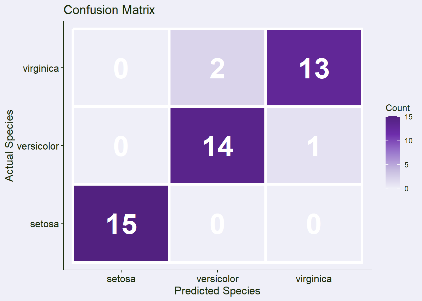

Feature importance

feature_importance <- data.frame(
  feature = rownames(importance(model)),
  importance = importance(model)[, "MeanDecreaseGini"]
) %>%
  arrange(desc(importance))

feature_importance |> 
  gt() |> 
  tab_header(title = "Feature Importance") |>
  fmt_number(columns = importance, decimals = 4) |> 
  table_theme()

feature	importance
Feature Importance
Petal.Length	30.8052
Petal.Width	29.6161
Sepal.Length	6.9387
Sepal.Width	1.8772

Plot 2: Feature Importance

importance_plot <- ggplot(feature_importance, 
                         aes(x = reorder(feature, importance), y = importance)) +
  geom_col(alpha = 0.8, fill = color_palette$discrete1[1]) +
  coord_flip() +
  labs(title = "Feature Importance in Random Forest Model",
       x = "Feature",
       y = "Importance Score")  +
  theme(plot.title = element_text(hjust = 0.5))

importance_plot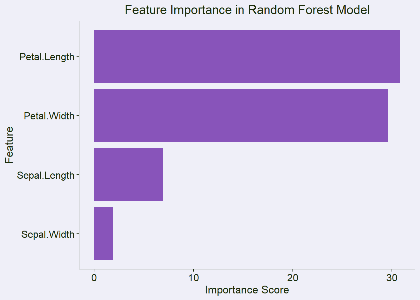

Create predictions DataFrame for visualization

test_results <- as.data.frame(X_test)
colnames(test_results) <- colnames(X)
test_results$actual <- y_test
test_results$predicted <- y_pred
test_results$correct <- test_results$actual == test_results$predicted

Plot 3: Prediction Results (using first two features)

prediction_plot <- ggplot(test_results, 
                         aes(x = Sepal.Length, y = Sepal.Width, 
                             color = predicted, shape = actual)) +
  scale_color_manual(values = color_palette$discrete1) +
  geom_point(size = 4, alpha = 0.7) +
  labs(title = "Model Predictions on Test Set",
       x = "Sepal Length (cm)",
       y = "Sepal Width (cm)",
       color = "Predicted",
       shape = "Actual") +
  theme(plot.title = element_text(hjust = 0.5))

prediction_plot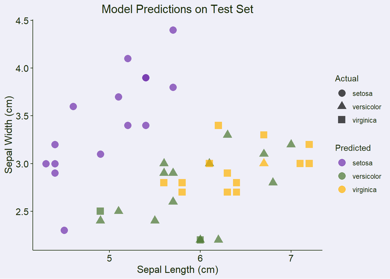

Save the model and preprocessing parameters to disk

saveRDS(model, "iris_rf_model.rds")
saveRDS(scaling_params, "iris_scaler.rds")